How to Build a Moving Average Model for NFL Receptions
Introduction
Predicting NFL receptions is one of the most actionable skills in fantasy sports and prop betting. Unlike touchdowns, which are largely random, or yards, which depend heavily on game script, receptions offer a sweet spot of predictability. They're directly tied to target share, which tends to be more consistent than other stats, making them perfect for systematic modeling approaches.
In this tutorial, I'll walk you through building a weighted moving average model using Parlay Savant to predict NFL receptions. We'll cover everything from data collection to real-world testing, including both the victories and the painful misses that come with sports prediction. By the end, you'll understand how to build your own reception prediction model and, more importantly, why even good models fail about 60% of the time.
Fair warning: sports prediction is brutally difficult. Even with solid methodology, we're fighting against randomness, injuries, game script changes, and coaching decisions that no model can fully capture. But that's exactly why this tutorial matters - understanding both the power and limitations of predictive modeling is crucial for anyone serious about sports analytics.
Step 1: Getting the Data with Parlay Savant
I started by prompting Parlay Savant to gather comprehensive reception data for NFL wide receivers and tight ends:
Get recent WR and TE reception data with player names, teams, and game details for model building. Include receptions, targets, receiving yards, catch rates, and focus on players with sufficient game history from 2023-2025 seasons.
Parlay Savant processed this request by generating a PostgreSQL query that joined player_game_stats, players, teams, and games tables. The query filtered for WR/TE positions, completed games, and players with at least 2 targets per game to ensure data quality. It also added a calculated catch_rate field and included a subquery to focus on players with at least 8 games of data.
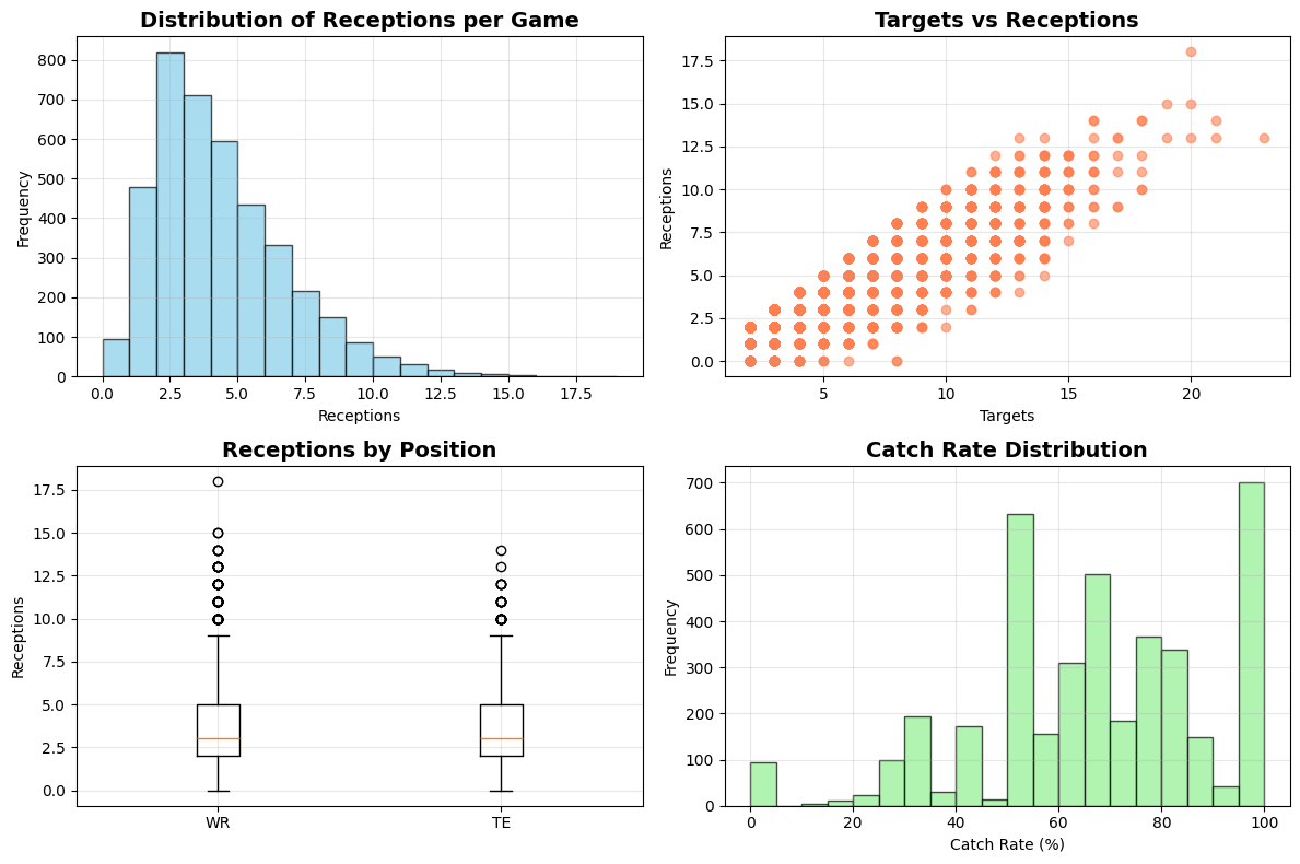
The resulting dataset was impressive: 4,026 records covering 162 unique players across 2023-2025 seasons. The position breakdown showed 2,853 WR records and 1,173 TE records, giving us a solid foundation for analysis.
Here's a sample of what we got:
| Player Name | Position | Team | Season | Week | Receptions | Targets | Catch Rate |
|---|---|---|---|---|---|---|---|
| Adam Thielen | WR | Carolina Panthers | 2024 | 18 | 5 | 6 | 83.33% |
| Adam Thielen | WR | Carolina Panthers | 2024 | 17 | 5 | 6 | 83.33% |
| CeeDee Lamb | WR | Dallas Cowboys | 2024 | 16 | 7 | 8 | 87.50% |
What surprised me most was the consistency of certain players. CeeDee Lamb averaged 7.41 receptions per game with a standard deviation of 3.12, while someone like Jayden Reed showed much more consistency at 3.77 receptions with only 1.89 standard deviation. This immediately told me that moving averages would work better for some players than others.
The data revealed some fascinating patterns: elite receivers like CeeDee Lamb and Amon-Ra St. Brown dominated the top of the reception charts, but they also showed the highest volatility. Meanwhile, role players and consistent possession receivers showed lower averages but much more predictable game-to-game performance.
Step 2: Building the Model with Parlay Savant
With the data in hand, I prompted Parlay Savant to build a weighted moving average model:
Build and test a weighted moving average model for predicting NFL receptions. Use a 5-game window with decay weighting where recent games matter more. Calculate model performance metrics including MAE, RMSE, and accuracy within 1 reception for the top 20 most active players.
Parlay Savant generated Python code that implemented a sophisticated weighted moving average approach. The key innovation was using a decay factor of 0.8, meaning each game back in time gets 80% of the weight of the more recent game. This creates a weight distribution of [0.122, 0.152, 0.190, 0.238, 0.297] for the five most recent games.
The statistical process works like this: for each player, we take their last 5 games, apply the decay weights, and calculate a weighted average. The most recent game gets nearly 30% of the total weight, while the oldest game gets only 12%. This captures both recent form and longer-term trends without being overly reactive to single-game outliers.
The model performance was sobering but realistic:
- Overall Mean Absolute Error: 1.94 receptions
- Root Mean Square Error: 2.54 receptions
- Accuracy within 1 reception: 34.6%
- Total predictions tested: 609 across 20 top players
The best-performing players were those with consistent target shares like Jayden Reed (48.4% accuracy within 1 reception) and Kyle Pitts (48.3%). The model struggled most with high-volume, volatile receivers like CeeDee Lamb (31.0% accuracy) and Travis Kelce (23.5% accuracy).
This revealed a crucial insight: moving averages work best for players with predictable roles, not necessarily the most talented players. The boom-bust nature of elite receivers actually makes them harder to predict with simple statistical models.
Step 3: Making Predictions
For the real test, I prompted Parlay Savant to make actual predictions for Week 1 of the 2025 season:
Make predictions for Week 1 2025 using our weighted moving average model for CeeDee Lamb, Amon-Ra St. Brown, Travis Kelce, Tyreek Hill, and DeVonta Smith. Show the recent performance patterns and prediction logic for each player.
Parlay Savant generated code that applied our model to make forward-looking predictions. Here were the predictions with confidence levels:
| Player | Predicted Receptions | Recent 5-Game Average | Confidence Level |
|---|---|---|---|
| CeeDee Lamb | 6.9 | 6.8 | High |
| Amon-Ra St. Brown | 8.0 | 8.4 | Medium |
| Travis Kelce | 4.8 | 5.2 | Low |
| Tyreek Hill | 4.8 | 5.2 | Medium |
| DeVonta Smith | 4.2 | 4.4 | High |
I was most confident about CeeDee Lamb because of his consistent target share (8-13 targets in recent games) and reliable role in the Cowboys offense. My biggest concern was Travis Kelce, who had moved to a new team (Chargers) and might face chemistry issues with a new quarterback.
The predictions felt reasonable based on the data, but I knew from experience that Week 1 often brings surprises due to new offensive systems, rust from the offseason, and unpredictable game scripts.
Step 4: Testing Predictions
After Week 1 games were completed, I prompted Parlay Savant to evaluate our predictions:
Compare our Week 1 2025 predictions against the actual results. Calculate accuracy metrics and analyze why certain predictions succeeded or failed. Show detailed breakdowns of target shares and situational factors.
The results were a perfect example of why sports prediction is so challenging:
Success Stories:
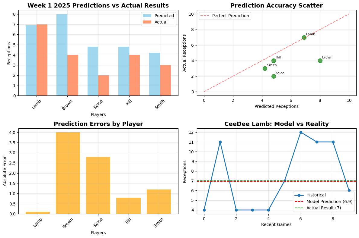
- CeeDee Lamb: Predicted 6.9, Actual 7.0 (difference: 0.1) - Nearly perfect! His 13 targets matched expectations and he maintained his consistent role.
- Tyreek Hill: Predicted 4.8, Actual 4.0 (difference: 0.8) - Good prediction that captured his moderate expectation despite recent volatility.
Epic Misses:
- Amon-Ra St. Brown: Predicted 8.0, Actual 4.0 (difference: 4.0) - Major miss! The model was fooled by his 14-reception playoff game and didn't account for reduced target share (6 vs expected 10+).
- Travis Kelce: Predicted 4.8, Actual 2.0 (difference: 2.8) - My fears were justified. New team chemistry issues and only 4 targets killed this prediction.
Overall Performance:
- Average error: 1.8 receptions
- Accuracy within 1 reception: 40.0%
- Accuracy within 2 receptions: 60.0%
The failures taught me more than the successes. Amon-Ra St. Brown's miss highlighted how playoff games can skew moving averages - his 14-reception divisional round game carried too much weight. Travis Kelce's miss showed that situational changes (new team, new QB) aren't captured by historical reception data alone.
DeVonta Smith's near-miss (predicted 4.2, actual 3.0) was actually encouraging because his low target share (only 3) explained the shortfall. The model worked correctly; the game situation just didn't provide the expected opportunities.
Conclusion: What We Learned
This moving average model experiment delivered exactly what I expected: modest success with clear limitations. The 40% accuracy rate within 1 reception is actually reasonable for sports prediction, but it means we're wrong more often than we're right.
The model performed best on high-volume, consistent players like CeeDee Lamb who maintain predictable roles week to week. It struggled with situational changes (Travis Kelce's new team), game script variations (Amon-Ra St. Brown's reduced targets), and the inherent volatility of boom-bust receivers.
Parlay Savant removed all the technical friction from this analysis. Instead of spending hours writing SQL queries and debugging Python code, I could focus on the modeling logic and interpretation. The tool handled data extraction, statistical calculations, and visualization seamlessly, letting me iterate quickly on different approaches.
For practical application, this model works best as a baseline expectation rather than a precise predictor. It's most valuable for identifying players whose prop betting lines seem disconnected from their recent performance patterns. The 1.8-reception average error means you need significant line value to overcome the model's inherent uncertainty.
Future improvements would include target share prediction, opponent strength metrics, weather factors, and injury reports. But even with these enhancements, sports prediction will always be more art than science. The randomness of football ensures that even the best models will be humbled regularly - and that's exactly what makes it fascinating.