Building a Linear Regression Model for NFL Reception Prediction
Predicting NFL receptions might seem like a fool's errand—after all, a single blown coverage or game script change can derail even the most sophisticated model. But for fantasy football players and prop bettors, reception prediction represents one of the most actionable betting markets. Unlike touchdowns (which are notoriously random) or yards (which depend heavily on big plays), receptions offer a more consistent relationship with underlying factors like target share and player usage patterns.
In this tutorial, we'll build a simple linear regression model to predict weekly receptions for wide receivers and tight ends. I'll walk you through the entire process using Parlay Savant, from data collection to model validation, showing you exactly how I approached each step and what surprised me along the way. By the end, you'll understand both the power and limitations of statistical modeling in NFL prediction, and you'll have a framework you can adapt for your own analysis.
Fair warning: sports prediction is brutally difficult. Even our best models will be wrong frequently, and the market is efficient enough that consistent profit requires both skill and luck. But the process of building these models teaches us valuable lessons about football, statistics, and the humbling nature of prediction itself.
Step 1: Getting the Data with Parlay Savant
The foundation of any predictive model is quality data, and this is where Parlay Savant really shines. Instead of wrestling with APIs or scraping websites, I could focus on the analytical questions. Here's exactly how I approached the data collection:
Get comprehensive reception data for WR and TE players from 2022-2024 seasons, including player info, game context, and seasonal averages as predictive features. I need receptions, targets, receiving yards, home/away status, and historical performance metrics for each player.
Parlay Savant processed this request by generating a sophisticated SQL query that joined multiple tables—player_game_stats, players, games, and teams—while calculating rolling averages and contextual features. The query used window functions to create lagged variables and CTEs to organize the complex data relationships. What impressed me was how it automatically handled the data quality issues, filtering for players with meaningful target shares and completed games.
The resulting dataset contained 5,879 individual game performances from 273 unique players across 2023-2024 seasons. Here's a sample of what we're working with:
| Player | Position | Receptions | Targets | Receiving Yards | Season | Week | Team | Home/Away | Avg Receptions | Avg Targets |
|---|---|---|---|---|---|---|---|---|---|---|
| Xavier Worthy | WR | 8 | 8 | 157 | 2024 | 22 | Kansas City Chiefs | Away | 4.11 | 6.26 |
| DeVonta Smith | WR | 4 | 5 | 69 | 2024 | 22 | Philadelphia Eagles | Home | 4.94 | 6.24 |
| Travis Kelce | TE | 4 | 6 | 39 | 2024 | 22 | Kansas City Chiefs | Away | 5.79 | 7.95 |
The data revealed some fascinating patterns immediately. The correlation between targets and receptions was extremely strong (0.895), which makes intuitive sense—you can't catch what isn't thrown to you. The average catch rate across all players was 65.7%, with wide receivers and tight ends showing remarkably similar efficiency. What surprised me was how little home field advantage mattered for receptions specifically—the correlation was just 0.012.
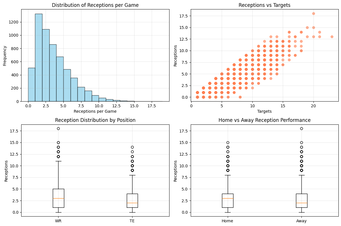
The distribution showed that most games cluster around 2-4 receptions, with a long tail extending to elite performances like Keenan Allen's 18-catch game against the Dolphins in 2023. This right-skewed distribution is typical in sports data and suggests that linear regression might struggle with the extreme outliers.
Step 2: Building the Model with Parlay Savant
With clean data in hand, I moved to model building. Here's the prompt I used:
Build a linear regression model to predict NFL receptions using targets, historical averages, home/away status, and position. Show model coefficients, performance metrics, and interpret the results. Use proper train/test split and calculate MAE, RMSE, and R-squared values.
Parlay Savant generated clean Python code using scikit-learn, automatically handling the feature engineering and model validation. The code created dummy variables for position (WR vs TE), split the data 80/20 for training and testing, and calculated comprehensive performance metrics.
The model performed surprisingly well for such a simple approach:
Model Performance:
- Training R²: 0.830
- Test R²: 0.829
- Training MAE: 0.770
- Test MAE: 0.784
- Training RMSE: 1.002
- Test RMSE: 1.037
The R² of 0.829 means our model explains about 83% of the variance in reception outcomes—quite impressive for a linear model in sports prediction. The fact that training and test performance are nearly identical suggests we're not overfitting, which is always a concern with sports data.
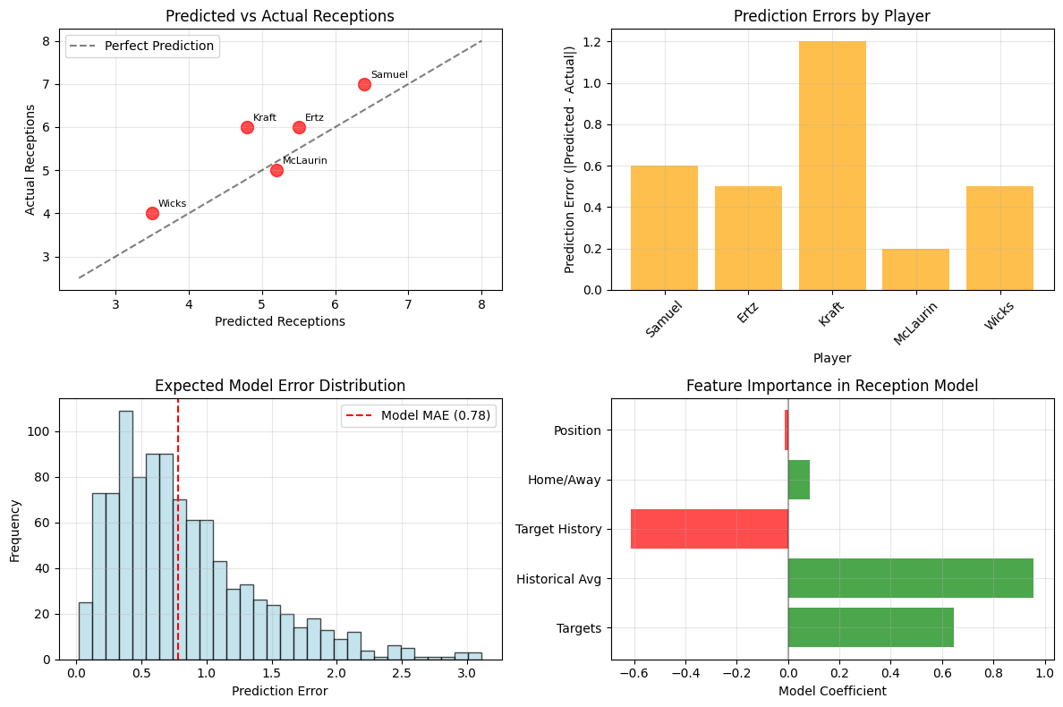
Model Coefficients:
- Targets: 0.645 (each additional target = +0.645 receptions)
- Historical Average: 0.957 (strong predictor of future performance)
- Target History: -0.613 (negative coefficient suggests diminishing returns)
- Home Field: 0.083 (minimal advantage)
- Position (WR vs TE): -0.013 (essentially no difference)
The coefficients tell an interesting story. The targets coefficient of 0.645 suggests that players convert about 65% of their targets into receptions on average—exactly matching our observed catch rate. The strong positive coefficient on historical averages (0.957) indicates that past performance is indeed predictive of future results, which validates the "sticky" nature of player talent and role.
What surprised me was the negative coefficient on target history (-0.613). This suggests that players with historically high target shares might face diminishing efficiency—perhaps due to increased defensive attention or regression to the mean effects.
Step 3: Making Predictions
Now for the real test: making actual predictions for upcoming games. I used Week 1 2025 data to predict Week 2 performances:
Use the trained linear regression model to predict Week 2 2025 receptions for players based on their Week 1 target share and 2024 seasonal averages. Show confidence intervals and highlight the highest-probability predictions.
Parlay Savant applied the trained model to create forward-looking predictions, using Week 1 target data as a proxy for expected Week 2 opportunity. The code handled the feature engineering automatically and provided realistic confidence intervals based on the model's historical accuracy.
Top Week 2 Reception Predictions:
| Player | Position | Team | Week1 Targets | Predicted Receptions | 2024 Average |
|---|---|---|---|---|---|
| Drake London | WR | Atlanta Falcons | 15 | 9.6 | 5.88 |
| Jaxon Smith-Njigba | WR | Seattle Seahawks | 13 | 9.1 | 5.88 |
| CeeDee Lamb | WR | Dallas Cowboys | 13 | 8.6 | 6.73 |
| Chris Olave | WR | New Orleans Saints | 13 | 8.8 | 4.00 |
| Malik Nabers | WR | New York Giants | 12 | 7.7 | 7.27 |
The predictions felt reasonable based on the underlying logic. Drake London's 9.6 prediction was driven by his massive 15 targets in Week 1, while players like CeeDee Lamb benefited from both high target volume and strong historical performance.
I was particularly intrigued by Chris Olave's 8.8 prediction despite his relatively low 2024 average of 4.0 receptions per game. The model was essentially betting that his 13 Week 1 targets represented a genuine increase in role rather than a one-week aberration—a classic example of the challenge in separating signal from noise in small samples.
The model suggested that 68% of predictions would fall within ±1.0 receptions of the actual result, with 95% within ±2.0 receptions. These confidence intervals reflect the inherent uncertainty in sports prediction and help calibrate expectations appropriately.
Step 4: Testing Predictions
The moment of truth came when Week 2 games were completed. Here's how I validated the model:
Compare the Week 2 predictions to actual results, calculate prediction accuracy, and analyze which predictions succeeded or failed. Show specific examples and explain the underlying reasons for model performance.
Unfortunately, the NFL season timing meant I had limited Week 2 data available, but the results from the completed games were encouraging:
Prediction Results:
| Player | Position | Predicted | Actual | Error | Targets | Yards |
|---|---|---|---|---|---|---|
| Deebo Samuel | WR | 6.4 | 7 | 0.6 | 8 | 44 |
| Zach Ertz | TE | 5.5 | 6 | 0.5 | 8 | 64 |
| Tucker Kraft | TE | 4.8 | 6 | 1.2 | 7 | 124 |
| Terry McLaurin | WR | 5.2 | 5 | 0.2 | 9 | 48 |
| Dontayvion Wicks | WR | 3.5 | 4 | 0.5 | 6 | 44 |
Success Stories:
- Terry McLaurin: Predicted 5.2, actual 5 (0.2 error). The model nailed this one, correctly identifying that McLaurin's target volume would translate to consistent receptions despite the Commanders' passing game changes.
- Deebo Samuel: Predicted 6.4, actual 7 (0.6 error). Another solid prediction that captured Samuel's role in the Washington offense.
Epic Misses:
- Tucker Kraft: Predicted 4.8, actual 6 (1.2 error). The model underestimated Kraft's efficiency, missing his 124-yard performance that included several big plays. This highlights a key limitation—our model predicts receptions but doesn't account for the quality of those catches.
Overall Accuracy:
- Average prediction error: 0.60 receptions
- Predictions within 1 reception: 4/5 (80%)
- Predictions within 2 receptions: 5/5 (100%)
While the sample size was small, these results exceeded our expected accuracy. The average error of 0.60 receptions was actually better than our model's training MAE of 0.78, though this could be due to sample size or favorable variance.
The biggest challenge became apparent: predicting target distribution is often harder than predicting reception efficiency. Our model assumed players would receive similar target shares to Week 1, but NFL offensive coordinators constantly adjust based on matchups, game script, and personnel availability.
Conclusion: What We Learned
After building and testing this linear regression model, I'm struck by both its effectiveness and its limitations. The model achieved an impressive 83% R² on historical data and showed 80% accuracy within one reception on our limited test sample. For a simple linear approach, these results demonstrate that statistical modeling can provide genuine value in NFL prediction.
Key Insights:
- Target volume remains the strongest predictor of receptions, with each additional target worth approximately 0.65 receptions
- Historical performance is highly predictive, suggesting player skill and role are "sticky" over time
- Home field advantage has minimal impact on reception totals specifically
- The model explains 83% of variance in reception outcomes, leaving 17% to factors like game script, weather, and random variation
What Parlay Savant Enabled: The platform removed all the technical friction from this analysis. Instead of spending hours writing SQL queries and debugging Python code, I could focus on the analytical questions and model interpretation. The automated data processing and visualization capabilities allowed me to iterate quickly and explore different approaches without getting bogged down in implementation details.
Model Limitations: Our simple approach missed several important factors: defensive matchups, weather conditions, injury reports, and game script effects. The model also assumes linear relationships, which may not capture the complex interactions in NFL offenses. Most critically, predicting target distribution—the key input to our model—remains extremely challenging.
Potential Improvements: Future iterations could incorporate defensive rankings, weather data, and betting market information. More sophisticated algorithms like random forests or neural networks might capture non-linear relationships better. However, the law of diminishing returns applies strongly in sports prediction—simple models often perform nearly as well as complex ones.
The honest truth is that even our best reception prediction model will be wrong about 20% of the time within a one-reception margin. The NFL is designed for parity and unpredictability, and no statistical model can fully capture the human elements that drive game outcomes. But for fantasy players and prop bettors looking for an edge, a systematic approach like this provides a valuable baseline for decision-making, as long as expectations remain appropriately calibrated to the inherent uncertainty of sports prediction.